Hip Hop’s 2023 Heavyweights

With over 15 million listeners, Spotify’s RapCaviar has been called “the most influential playlist in music.” RapCaviar is curated by Spotify’s editorial team and updated daily to represent the latest and greatest hip-hop and rap tracks.

For the last year, I’ve saved a daily snapshot of the playlist using the Spotify API to empirically determine the biggest rappers in hip hop today. In this post, we’ll use hard data to approximate influence, hustle, and longevity for rap’s biggest names during 2023.

Methodology

To collect the data, I scheduled a Python script to run daily to (1) hit Spotify’s API to collect the RapCaviar track list and (2) save the resulting data frame as a .csv file to an S3 bucket. After pulling down and combining all daily files from S3 using an R script, the tidied dataset contains 11 fields:

Field NameSample Value
Playlist Id37i9dQZF1DX0XUsuxWHRQd
Playlist NameRapCaviar
Track Playlist Position2
Track NameMad Max
Track Id2i2qDe3dnTl6maUE31FO7c
Track Release Date2022-12-16
Track Added At2022-12-30
Artist Track Position1
Artist NameLil Durk
Artist Id3hcs9uc56yIGFCSy9leWe7
Date2023-01-02
The value for “artist track position” helps distinguish owners from features. For example, both Lil Durk and Future participate in the track Mad Max. Since it’s Lil Durk’s song and Future is the feature, a two row exists in the dataset, with values of “artist track position” set to 1 (Lil Durk) and 2 (Future).

After the cleaning and duplication process, the dataset contains 469 total tracks with 271 distinct artists represented across 351 distinct playlist snapshots between January 1 to December 27, 2023.

Metrics

Influence

Let’s start with influence: what percent of available days was a given artist represented on the playlist? For example, if an artist appeared in 50 of the 351 possible daily snapshots, their “influence” score would be 14.2%.

Here are the top ten rappers ranked by this influence metric, for 2023:

NameDays RepresentedPercent of Available
Drake351100%
Future351100%
Gucci Mane351100%
Travis Scott351100%
21 Savage34498%
Kodak Black33094%
Yeat32893%
Latto31189%
Lil Uzi Vert30988%
Quavo30286%

Impressively, four artists yielded sufficient influence to maintain a presence on the playlist every day of the year: Drake, Future, Gucci Mane, and Travis Scott. Here’s a visual representation of their dominant year:
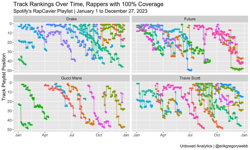
Each colored line represents a unique track. With the y-axis reversed, the chart shows how new tracks enter the playlist positioned near the top and then descend over time. The biggest surprise to me is Gucci Mane, who managed to maintain his presence on the playlist via 14 distinct tracks released throughout the year:
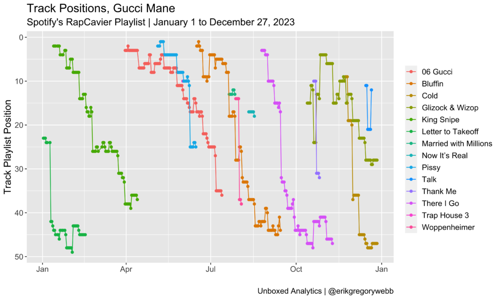
The hustle shown here reminds me of my favorite Lil Wayne clip of all time.

Notably, 21 Savage was only a week short of full coverage, coming in at 98%.

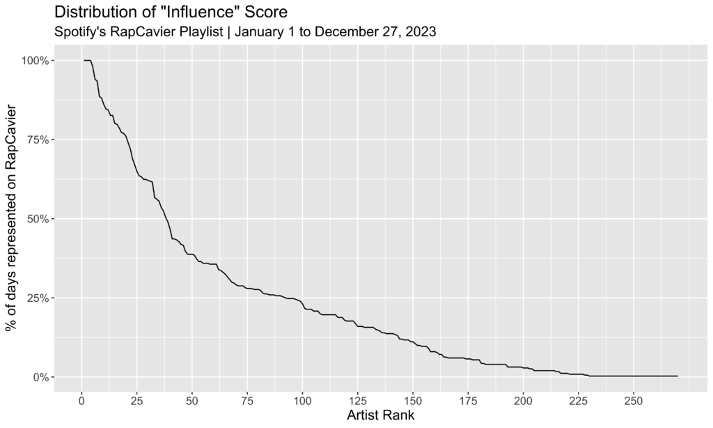
Looking at the distribution of influence scores for all artists appearing at least once during the year, 38 (14%) were present in the RapCaviar playlist more than half of the year:
Density

It’s one thing for an artist to have one of their tracks represented on RapCaviar, but the heavyweights often have several at once. “Density” is calculated as a distinct count of tracks by artist and day.

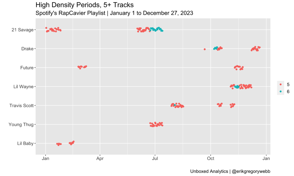
The highest density score for 2023 was 6, a score achieved by just four rappers:

DensityArtist | Dates
6 tracks21 Savage | Jun 23 – Jul 13 (21 days)
6 tracksLil Wayne | Nov 10 – 16 (7 days)
6 tracksDrake | Oct 7 – 12 (6 days)
6 tracksTravis Scott | Aug 3 (1 day)

Most impressive is 21 Savage’s dominant 21-day, 6-track run over the summer, preceded by a 20-day, 5-track run. Notably, during the 6-track spree, all six were features or joint tracks:

  1. Pull Up (feat. 21 Savage)
  2. Wit Da Racks (feat. 21 Savage, Travis Scott & Yak Gotti)
  3. Peaches & Eggplants (feat. 21 Savage)
  4. 06 Gucci (feat. DaBaby & 21 Savage)
  5. War Bout It (feat. 21 Savage)
  6. Spin Bout U (with Drake)

Contributing to more than 10% of the playlist’s track count simultaneously is truly impressive (RapCaviar usually has 50 tracks total); rap’s heavyweights are dense.

Longevity

Finally, let’s consider longevity, meaning how long an artist’s tracks remains on the playlist. Here are the top ten songs by lifespan on the RapCaviar track list during ’23:

TrackArtistDaysFirst DayLast Day
f*kumeanGunna179Jun 19Dec 14
Turn Yo Clic UpQuavo167Jul 14Dec 27
Search & RescueDrake161Apr 7Sep 15
500lbsLil Tecca159Jul 21Dec 27
I KNOW ?Travis Scott153Jul 28Dec 27
Paint The Town RedDoja Cat146Aug 4Dec 27
MELTDOWNTravis Scott143Aug 1Dec 21
Private LandingDon Toliver136Feb 24Jul 13
SuperheroMetro Boomin135Jan 2May 25
All My LifeLil Durk133May 12Sep 21

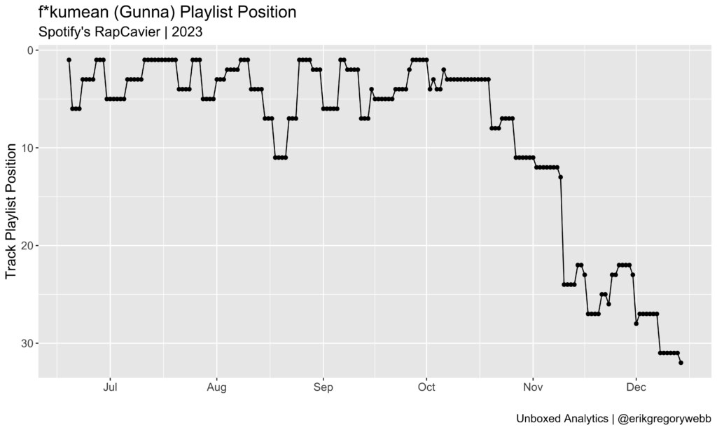
Importantly, four of the tracks in the top ten are still active (italicized above), so there’s a decent chance Turn Yo Clic Up could outlive f*kumean. Speaking of which, Gunna’s first top-ten solo single managed to spend almost six months on RapCaviar, complete with a position surge in mid-August:
Zooming in, here’s the position history for all of those top ten tracks:
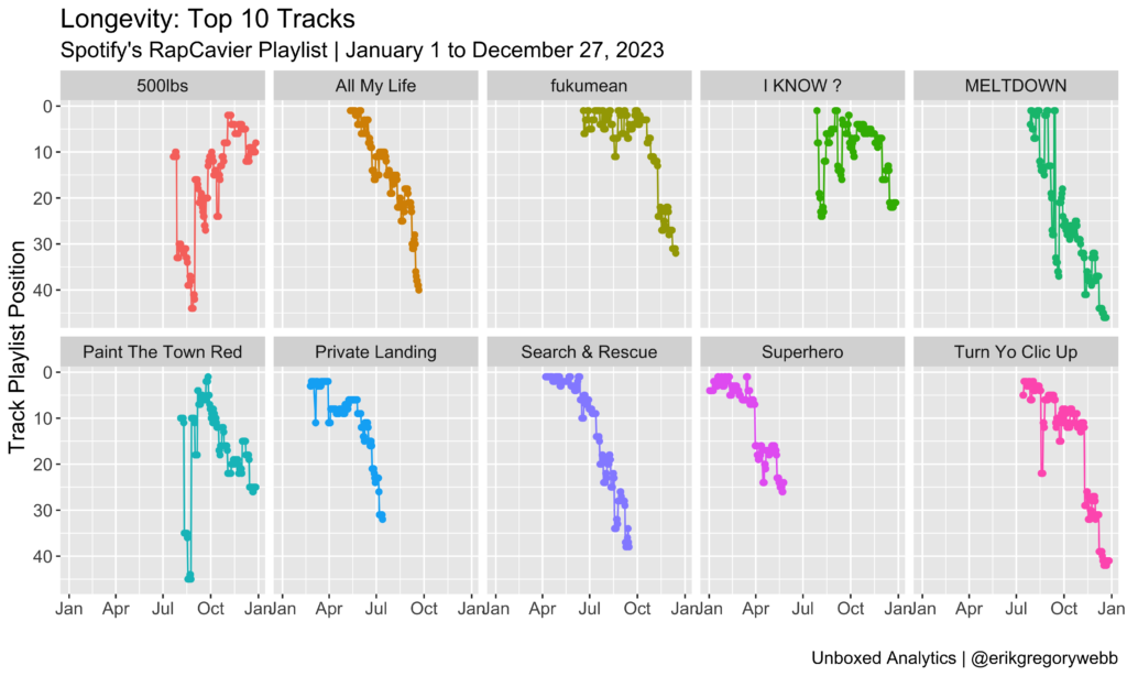
Most of the time, a track will debut on the playlist and then fade out over time, sinking deeper in the set list before falling off. Good examples are All My Life, Private Landing, and Search & Rescue. Hits like 500lbs and Paint The Town Red are more anomalous, with momentum building within the playlist over time.

To close this metric out, let’s look at the top ten rappers with the highest average longevity per track, for those artists with three or more distinct tracks ever appearing on the playlist during the year:

NameMedian LongevityAverage LongevityTrack Count
Gunna1161034
Metro Boomin92966
Ice Spice96724
Latto75744
Moneybagg Yo75696
Lil Uzi Vert68648
Don Toliver41645
Toosii79633
Key Glock61624
Sexyy Red63624
Conclusion

The influence and density metrics point toward the same heavyweights: 21 Savage, Drake, and Travis Scott. This is intuitive since the two metrics are correlated. The longevity metric shines the spotlight on a different subset of rappers, like Gunna, Metro Boomin, and Ice Spice.

Either way, it was a great year for rap. Thanks for reading!

Visualizing Rap Communities with Python & Spotify’s API

Finding new music you like can be tough. In my experience, there’s no single discovery mechanism that delivers consistently. I usually rely on a mix of sources: websites like Pitchfork or Genius, subreddits like popheads or hiphodheads, and curated playlists like Get Turnt or Hot Rhythmic. Lately, I’ve found new favorites through a Spotify feature called “Fans Also Like”.

FANS ALSO LIKE – A Spotify music discovery feature

Listed on each artist page, the “Fans Also Like” section is an algorithmically populated discovery feature built using a metric called “artist similarity”. This metric is based on shared fans, meaning the more fans two artists have in common, the higher their similarity score.

“Artist similarity is probably the second-most important piece of data we extract from listening patterns—after popularity. It’s the data behind radio, genres, and Discover pages.”

Glenn McDonald, Spotify’s data alchemist (source)

The cool thing is that Spotify exposes this discovery algorithm via API. After authenticating and supply an artist id, the API will return a list of 20 similar artists. Obviously, this is a huge win for music data nerds everywhere.

In this post, I’ll leverage Spotify’s “similar artists” API to build interactive network charts, visualizing how artists are linked together, as measured by the similarity of their fans.

Walkthrough

To access the Spotify API, you’ll need a Spotify account (free or premium), and a registered application. To make things easy, I used the spotipy library in Python, which supports all of the features of the Spotify Web API.

Next, leaning on the the spotipy library to do the heavy lifting, I can retrieve the artist and “similar artist” data with two lines, passing the artist id to the artist and artist_related_artists functions.

Here’s a sample of the result when we query Spotify for the artists most similar to Drake, according to listener behavior:

NamePopularityFollower Count
Big Sean87 7,113,709
J. Cole90 10,379,858
Jeremih84 4,094,532
Wale80 2,457,939
Rick Ross86 3,839,127

The list of similar artists is returned in order of ranked similarity score, meaning that according to the listener data, Drake is most similar to Big Sean, J.Cole, and Jeremih. Surprising? Let’s make the list more visual by creating an interactive plot using Flourish.

It’s a fun visual, but you’d find these same faces if you looked at “Fans Also Like” on Drake’s artist page. Let’s take it a step further and query the API for similar artists for the artists similar to Drake. Then we’ll start to get a sense of the pop-rap landscape.

Right off, it looks like Jeremih is the odd one out, with none of his peer artists overlapping with the rest of the group. In contrast, Big Sean overlaps three of five, J.Cole, Wale, and Rick Ross, with Drake.

Let’s see how things look when we pull in the full dataset, with each of Drake’s top 20 most similar artists and each of their 20 most similar artists.

How could we use this data to find new music? Counting the number of times an artist appeared across the second iteration of similar artists, below are the top artists to check out if you’re a Drake fan:

This has been one approach to understanding “community” in rap music. Another would be to analyze collaboration between artists and the frequency of features shared. However you find new music, “Fans Also Like” is a fantastic tool to explore new artists, and even genres.

You can find the full code to create the dataset used here and the dataset itself here.
Building a Birthday Text Bot using Twilio

A good way to show family and friends you care is remembering their birthday. It seems simple enough but in practice, birthday tracking for anyone beyond immediate family and very close friends can be time consuming. Thankfully, you can automate that!

While outsourcing birthday check-in duties does feel a bit impersonal, you can always follow up on the generic message after getting a reply. This post is a tutorial for building a birthday text bot using Twilio.

The first step to building a birthday bot is storing the list of birthdays and contact information somewhere. In this example, I’ve used Coda.io to store name, birthday, and phone number. While I’d prefer to use Google Sheets, Coda’s API interface makes it very easy to import data into the Python environment. Authentication occurs via a bearer token and the API returns a JSON file.

After a bit of unpacking and cleaning, we have a birthday data frame like the one below (this is dummy data, for obvious privacy reasons).

Next, since this code will be deployed to a server and run on a daily schedule, we need to determine which, if any, of our family or friends is celebrating their birthday today.

Finally, we need to tap into the power of Twilio to send the actual SMS message. Twilio is a really cool API service that allows you to programmatically make phone calls and send or receive text messages.

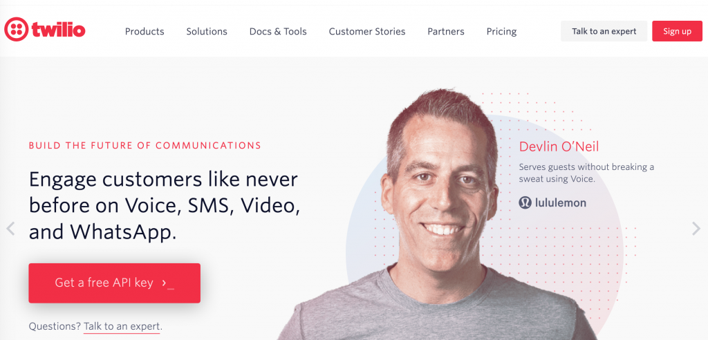
twilio.com

The actual code required to make the birthday bot come to life only requires about eight lines of code. After supplying an account identifier and authentication token, the message client takes as input the body of your text, your Twilio number, and the recipient’s phone number.

That’s it! Let’s see what the message looks like on the recipient’s end.

Very slick. By connecting a database (Coda.io) to a messaging API (Twilio), we’ve created a simple birthday text service, capable of earning you the reputation of most thoughtful friend. Enjoy!

Full code can be found on GitHub here.

Feature photo by Sarah Pflug from Burst.

Building a Simple Crypto Alert Bot in Python

Introduction

In the long run, I think cryptocurrencies will be more valuable than they are today, on average. The investment strategy consistent with that belief is to buy and hold (disclaimer below). However, considering a record of considerable volatility, could a crypto enthusiast be smarter about when to buy, in pursuit of a “bargain”?

This post outlines the process of building a simple crypto “bargain buy” alert system using Python, which sends a notification when a given cryptocurrency (BTC, XRP, ETH, etc.) appears “cheap” relative to historical prices. I use CoinAPI for current and historical cryptocurrency pricing and the Slack API for iOS and web push notifications.

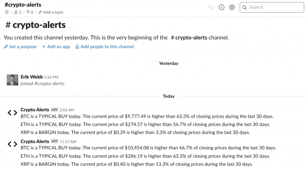
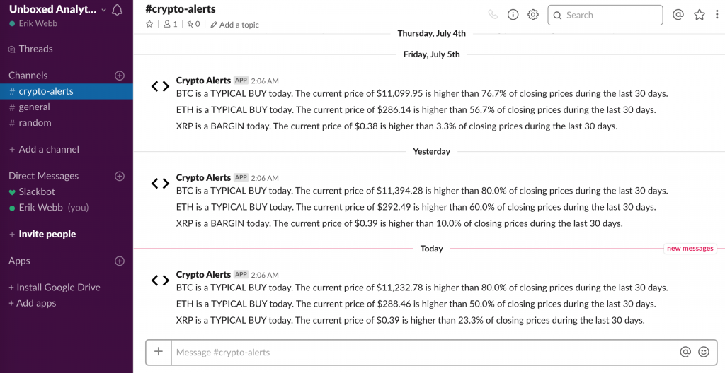
My “Crypto Alerts” Slack bot notifies me of “bargain” opportunities daily

The true focus here is not the specific strategy (i.e. determining the right time to buy) but rather, demonstrating how APIs can power the creation of new and valuable services.

I broke the alert system process into four pieces:

  • Retrieve the crypto’s current price (CoinAPI)
  • Retrieve the crypto’s historical price data (CoinAPI)
  • Determine if current price is a “bargain”
  • Summarize findings via push notification (Slack API)
CoinAPI offers a entry-tier API key with 100 free daily calls

After writing the script in Python, I deployed it to PythonAnywhere and scheduled it to run daily. With that overview in place, let’s dive in and walk through the details!

Code Walkthrough

As usual, we’ll start by bringing in the necessary libraries. We’ll use the request library to make the API calls (GET from CoinAPI and POST to the Slack API), the pandas library to organize the JSON response.

To start, we send a request to CoinAPI to retrieve the current price of the cryptocurrency, measured in USD.

To retrieve historical exchange rates, we’ll modify the URL and specify that we’d like daily values for the last 30 days. For simplicity, we can save the results into a pandas data frame.

Now that we have the current price and a historical benchmark, we can take a stab at determining if the cyrpto is a “bargain”.

My approach here is unsophisticated. If the current price is less than the 20% percentile of prices from the last 30 days, it’s considered a bargain. If it’s greater than the 80% percentile, it’s a “rip-off”.

This goes without saying, but this strategy won’t make you a Bitcoin millionaire! However, it does provide a basic alert bot framework.

When I ran this code while testing, at a price of $11,706, BTC was labeled as a rip-off. Here’s a sample of the message the bot produces:

BTC is a RIP-OFF today. The current price of $11,706.27 is higher than 83.3% of closing prices during the last 30 days.

Finally, the last piece of the alert system is to distribute the trading insight via a push notification. Luckily, this is pretty easily accomplished using the Slack API.

To leverage this free resource, I created a new domain and registered an application. This supplied the required authentication token.

Once automated through Python Anywhere, the messages look like this inside of my “crypto-alerts” channel. They are also conveniently pushed to my iPhone via the Slack mobile app.

You can find the complete script here. Thanks for reading!

Disclaimer: This content is for informational purposes only. Nothing contained here constitutes a solicitation, recommendation, endorsement, or offer to buy or sell any securities or other financial instruments (including cryptocurrencies) in this or in in any other jurisdiction.

Lessons from the Tank: Analyzing 800+ Shark Tank Pitches

Even though it’s been around for years, I just recently discovered Shark Tank, the show where hopeful entrepreneurs pitch business ideas to a panel of wealthy investors, or “sharks”. I usually wonder if there’s a method to the deal-making madness, especially when a pitch that resonates with me falls flat on the sharks.

In this post, I take my fandom to a deeper level by using episode descriptions from Wikipedia to understand what kinds of pitches have the highest chance of being offered a deal. In the process, I’ll use tools like web scraping, natural language processing, and API calls to gather, transform, enhance, and visual the data.

I’ve divided my workflow for this project into four steps:

  1. Obtain episode-level descriptions via web scraping
  2. Reshape data from episode-level to pitch-level
  3. Enhance data by categorizing descriptions via uClassify API
  4. Visualize key trends by season and pitch categories
“Follow the green, not the dream” – Shark & Billionaire Mark Cuban

1. Obtain episode-level descriptions via web scraping

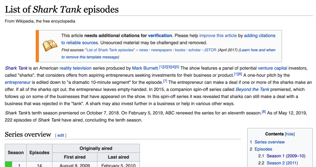
This analysis is possible because of a Wikipedia page that contains short descriptions of every pitch delivered on Shark Tank.

Wikipedia: List of Shark Tank Episodes

The first step is to extract this information via the rvest package in R, looping over each of the nine tables (corresponding to nine seasons) within the page.

Next we’ll do a bit of cleaning, simplifying column naming conventions, and adjusting the data types for the air date and viewership fields.

2. Reshape data from episode-level to pitch-level

In its current form, we won’t be able to detect any patterns with this data since the descriptions are bundled at the episode-level, like this:

“Crooked Jaw” a mixed martial arts clothing line (NO); “Lifebelt” a device that prevents the car from starting without the seat belt being fastened (NO); “A Perfect Pear” a gourmet food business (YES);

We need to “un-nest” the descriptions so that each row contains a single pitch. This is easily accomplished using the unnest function from tidyr.

Now we have a clean dataset, ready to enhance and analyze. Here’s a sample of the data structure, highlighting a few variables:

no_overallpitch_descriptiondeal
1a pie companyYES
2an implantable Bluetooth device requiring surgery to insert the device into the user's headNO
3an electronic hand-held device for waiting roomsNO
4a plastic elephant-shaped device that helps parents give small children oral medicineYES
5a packing and organizing service based on an already successful business called College Hunks Hauling JunkNO
6a mixed martial arts clothing lineNO
7a device that prevents the car from starting without the seat belt being fastenedNO
8a gourmet food businessYES
9a Post-It note arm for laptopsNO
10a musical way to teach students ShakespeareYES

3. Enhance data by categorizing descriptions via API

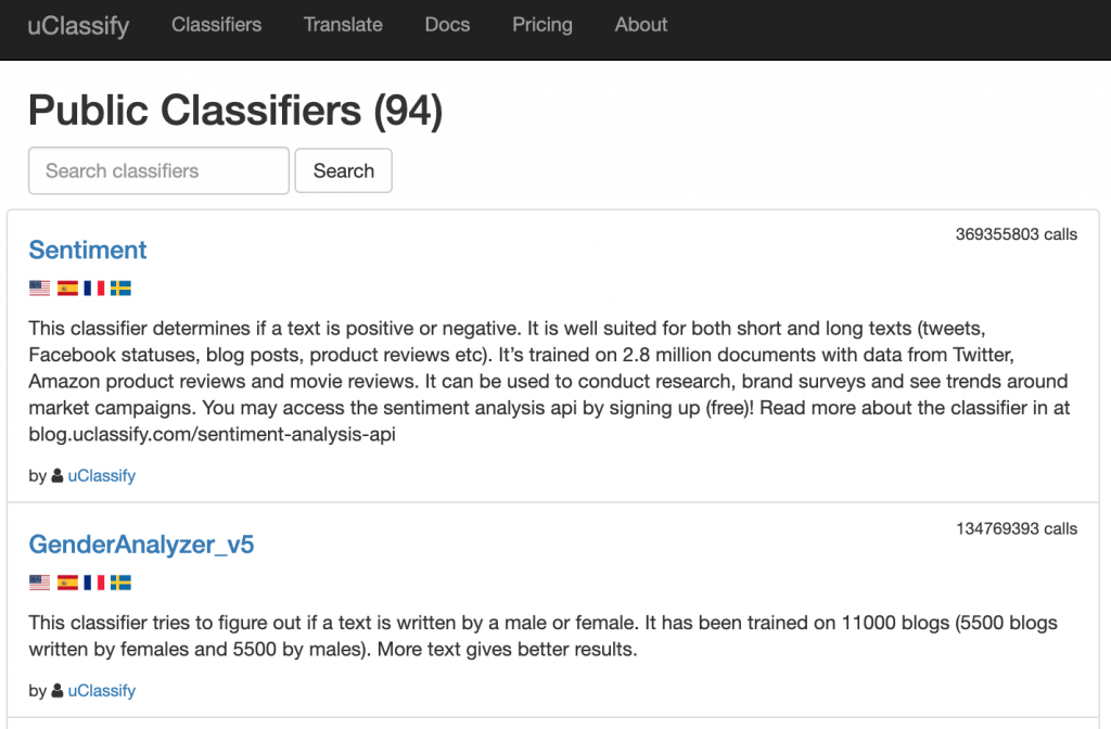
How can we systematically analyze what kind of pitches are more likely to be offered a deal when all we have is a brief text description? Rather than build my own NLP model from scratch to categorize pitches, I used uClassify, which offers “Classification as a Service” (CAAS).

Much like Google Cloud’s Natural Language API, uClassify provides on-demand NLP services via API. To categorize the Shark Tank pitches, I used the free “Topics” and “Business Topics” classifiers.

Let’s see how this was implemented in the R code:

These functions construct a URL with my personal API key, the classifier API name, and the text (pitch description) to be categorized. A GET call then returns a JSON with a list of categories and “match” scores.

For example, take pitch #803, “Thrive+”, which has this description: “capsules that reduce alcohol’s negative effects.” The category with the highest “match” score was Health, followed closely by Science. By categorizing the pitch descriptions, we’ll be more equipped to uncover some key elements of successful Shark Tank pitches.

Cheers (formally Thrive+) Landing Page

4. Visualize key trends by season and pitch categories

Now for the fun part! After compiling, cleaning, and enhancing our dataset, we’re ready to visualize and model the data. First, let’s take a look at Shark Tank’s popularity over time, measured in TV viewership (in millions).

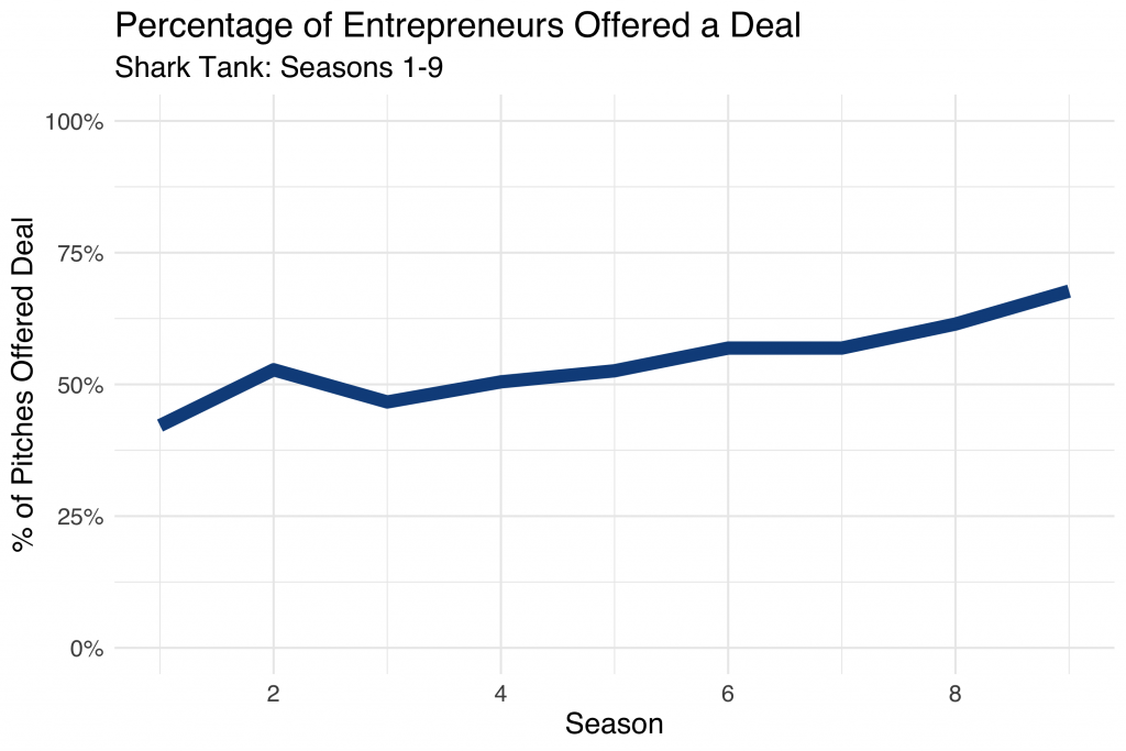
Even without the fitted line, it’s easy to see a rise and fall in popularity, with the peak around 2015 with 7.5 million viewers. Next, let’s look at how willing sharks were to make deals over the course of the show, across nine seasons:

During Season 1, less than 50% of pitches were offered a deal from the sharks. By season 9, deals were made over 65% of the time! I wonder if this had anything to do with sliding viewership.

Let’s dig a bit deeper and start looking at characteristics of successful pitches. Using the tidytext methodology, I determined which words within the pitch descriptions were most often associated with a strong response from the sharks (for better or worse).

WordDealNo DealNet
clothing715-8
portable103+7
bags71+6
cooking71+6
designed1610+6
ice17-6
car61+5
cleaning61+5
hair116+5
healthy50+5

Clothing is mentioned in 22 pitch descriptions, 70% of which were unsuccessful! On the flip side, when the pitch included something “portable”, the sharks were willing to make a deal 10 out of 13 times. If you make it onto Shark Tank, don’t mention ice! For whatever reason, almost 90% of those pitches resulted in no deal with the sharks.

Now let’s see what else we can learn by using the categories generated from the uClassify API classifiers:

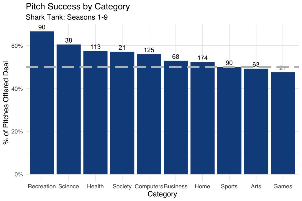
Here we summarize pitch success by category, with the total number of pitches within the category represented above each bar. The dashed grey line represents the 50% cutoff, where a pitch within a given category is equally likely to be accepted or rejected.

Notice how over 65% of deals classified as “Recreation” were offered a deal by the sharks over the course of the nine seasons. It looks like “Game” entrepreneurs didn’t snag funding quite as easily!

Conclusion

This has been a fun and quick way to explore some of the nuance in the world of Shark Tank deal-making. Truthfully, the dataset we created was pretty limited. Adding in information like which shark (or sharks) made the deal, for how much, and for what percentage of equity would add more precision compared to simply knowing if a deal was made or not.
In addition, access to full pitch transcripts (rather than simplistic descriptions of ~10 words or less) would be much more helpful in accurately classifying the pitches into meaningful categories.

You can find the complete R code here and the final dataset here, both hosted on GitHub. Thanks for reading!
Mapping Scarsdale Real Estate Data with Python

This year my wife and I moved to New York for the start of a new job. Initially overwhelmed by the scope and pace of the NYC housing market, we were given the very generous and unexpected opportunity by a family friend to live in a house north of the city in Westchester County. Built in the early 1930s, the historic home is situated in central Scarsdale, an affluent suburban town known for high-achieving schools and extravagant real estate.

As a graduate student of historic preservation, my wife has been especially enthralled by the rich styles and architecture of the houses within the Scarsdale village limits. Naturally, we frequently discuss and analyze the homes we pass on walks and runs, her comments generally centered around history and architecture, mine on economics and valuation.

Sourcing the Data

Wishing to analyze the houses of Scarsdale in a more systematic way, I began to experiment with the Zillow API. Disappointed by both accessibility and content, I continued to search for a superior data source. Soon after, I discovered a tool developed by the Village of Scarsdale to search property information by road name and wrote a Python script to scrape the data. Curious to know if additional variables were available, I contacted the Scarsdale Village administration and was sent an Excel file with the complete set of residential properties, rich with detail and with few missing values (5,000+ rows, 100+ columns).

The dataset includes the address of each residential property, but for visualization purposes, I needed geographic coordinates (latitude, longitude). Luckily, the Google Maps API provides this exact functionality, known as geocoding. Having some experience with this API, it was simple to write a Python script to retrieve the geographic coordinates for each of the 5,000 properties.

After writing an R script to scrub the data (creating more descriptive variable names, filtering, removing duplicates), I was ready to visualize the real estate data of America’s most affluent town.  You can find both the raw and cleaned datasets here.

Mapping the Data

After considering the many potential ways to map the properties, I settled on three key views: Year Built, Total Assessed Value, and Sales Date.

After some research, I discovered the folium library, which leverages the mapping strengths of the leaflet.js library within the Python ecosystem to provide Tableau-like functionally. The timing was ideal considering my free Tableau college subscription recently expired!

1. Year Built

With (a few) homes built as early as the 1600s and (some) as recently as 2018, this view shows clusters of homes built in similar time periods and paints a picture of development over time.

Here, the color spectrum plots blue for older houses and red for newer houses. Drag to interact with the map and click on a dot to view the address and year built.

Note the layers of development along the Saxon Woods Golf course border and the concentration of older homes in the Greenacres area.

Full Page Map: Link

2. Assessed Value

In this heatmap, the brighter the dot the higher the assessed value. Clicking on a circle reveals the total assessed value for the current tax year as well as the square footage of the home.

Full Page Map: Link

Sales Date

Which neighborhoods are hot on the market? This view maps the data according to sales date, with more recent sales colored in green. No clear trend emerges here, with a fairly equal distribution across the village. Clicking on a dot reveals the latest sales date and the number of years since sale.

Full Page Map: Link

Code Appendix

We’ll now dive into how these maps were created. As usual, we start by calling the necessary libraries. Beyond the essential pandas and numpy libraries, I use folium for map creation and matplotlib.cm for color assignment.

In order to visualize a feature such as assessed value or years since last sales date, I needed to be able to bucket the values and assign each bucket a color.

The function below achieves that need, allowing the user to specify the number of buckets and a color spectrum. BI software such as Tableau replicates this kind of functionality, but with superior algorithms that scale for large datasets.

Finally, below is the framework used to create each of the maps. A dot is created for each of the properties, colored according to the bucket assigned and labeled by year built, total assessed value, square footage, or sales date.

You can find the complete code to replicate these maps here and the dataset here. Thanks for reading!

Extracting Public Transactions from Venmo API with R

Public by default, your Venmo transactions are surprisingly accessible to anyone with an internet connection. Although Venmo has removed functionality to query historical transactions, it’s public API still provides a real-time snapshot view of transactions processed through the system, including usernames and payment subjects (though not the amount sent or received). Try it for yourself here.

With that said, it was straight-forward to collect a bit of data from this API using R. The bulk of the script was needed to parse the JSON file returned by the API to extract interesting information. In this post, I’ll highlight sample data from the API in an effort to expose the kind of information being openly shared. If you use Venmo, follow these instructions to change your transactions to private by default.

Sample Data

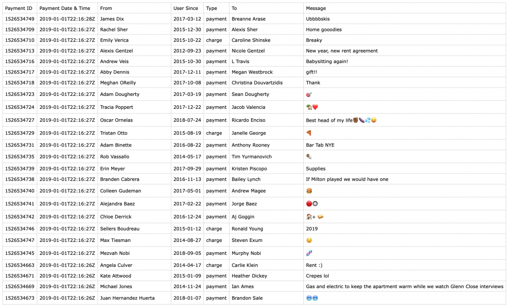
Using the API, I collected data from 1,250 payments. From each of these transactions, I was able to view the following information:

  • Payment Id
  • Payment Date, Time
  • Payment Message
  • Sender & Receiver Name, Username
  • Sender & Receiver Profile Photo
  • Sender & Receiver Venmo Account Creation Date

For example, on January 1, 2019 Scott Perkinson sent Patrick Miller an undisclosed payment for “Caroline Bachelorette Party & Wine tasting”. That same day, Kerry McCarthy paid Anna McCarthy for “Barbie dream house furniture.” You can’t make this stuff up.

Bottom line, privacy is important, and you should take any available steps to limit how your information is shared. If you use Venmo, start by making your payments private by default. You can find the datasets I compiled here and the R code to access the API here.

Using the Google Maps API to Visualize Chase’s Presence in Utah

I’ve been a happy Chase customer since 2010. I’ve appreciated the investment in their mobile platform and was excited about the recent You Invest announcement, allowing customers to trade 100 stocks and ETFs a year for free. With 5,100+ branches and 16,000 ATMs+ nationwide, Chase has a strong national footprint.

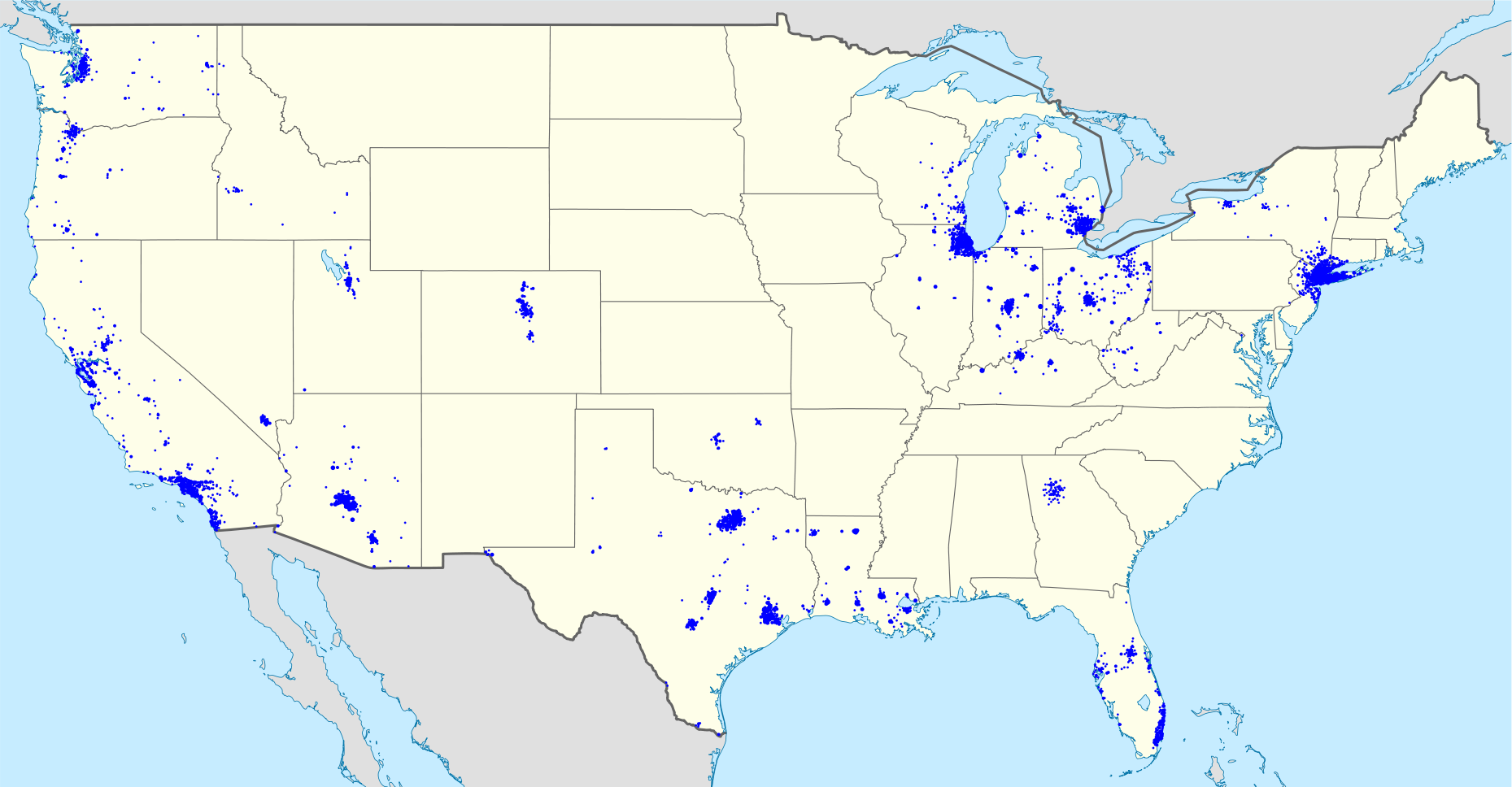
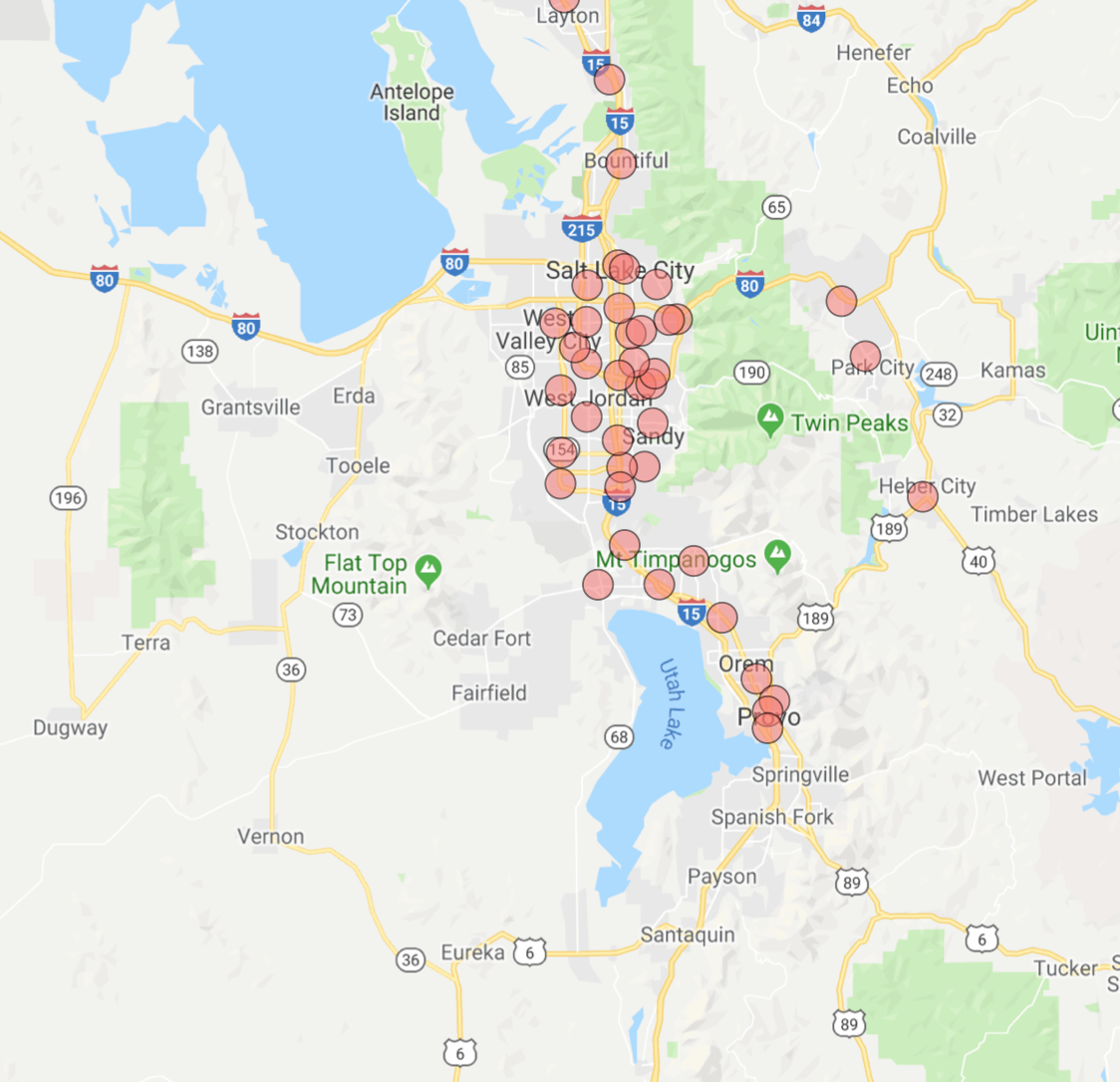
In this post, I use Python to recreate the map below for my home state of Utah, scrapping branch and ATM information from Chase.com and obtaining geographic coordinates using the Google Maps geocoding API.

chase-footprint
Chase branches in the U.S. in 2010. Source: Wikipedia

Before going further, I’d invite you to read Chase.com’s Terms of Use as well as Roberto Rocha’s article about the ethics of web scrapping. To avoid excessive server demands (although an unlikely issue for Chase), we’ll explicitly space out requests, made easy with Python’s time sleep method.

Scrapping Branch & ATM Information with Selenium

As usual, we’ll begin by calling the necessary libraries.

Next, we need to pass the driver a URL. Here I’ve used the Utah URL. This could easily be adapted to other states by changing the last two letters of the link.

Also note the executable path, which is pointed to the directory where my ChromeDriver is located. You can download the driver here.

When this code finishes running, the “locations” list contains location names, such as the following Utah cities:

We then convert these locations into Chase.com URLs.

The links now look like this:

The function below represents the process of scrapping the data for each location.

We’ll apply the function to each location URL to extract the corresponding branch and ATM information.

Finally, we’ll clean the information we’ve scrapped and organize it into tidy columns.

Here a sample of what the final dataset looks like:

LocationAddressType
Bountiful510 S 200 W Bountiful, UT 84010Branch
Farmington Station Park100 N Station Pkwy Farmington, UT 84025Branch
Brigham Young University800 E Campus Dr Provo, UT 84602ATM
Fashion Place6255 S State St Murray, UT 84107Branch

Geocoding Branch Address via Google Maps API

Per Google’s Get Started article, geocoding is the process of converting addresses into geographic coordinates, like latitude and longitude. Once we have a longitude and latitude combination, we can plot the branch and ATM locations on a map using Tableau or R.

Here is the Python code used to accomplish the geocoding:

Please note that you’d need to insert your own Google Cloud API key to make the code run. Finally, let’s visualize some of the data points with R!

Here’s the code to create this visualization:

You can view the data here and the complete code here. Thanks for reading!

Analyzing Drake’s Catalog Using Spotify’s API

I’ve been a Drake fan since 2009 when I first heard “Best I Ever Had” from So Far Gone. Over the last decade, I’ve watched Drake transform into a global rap and pop superstar. This weekend I saw Drake live in Brooklyn as part of the Aubrey & the Three Migos tour. What better way to celebrate than by analyzing his catalog using Spotify’s API? I’ve broken the celebration into two parts, getting the data and analyzing the data. Click here if you’d rather skip the code and jump into the analysis.

Getting the Data

In this post, I use Spotipy, “a lightweight Python library for the Spotify Web API”. Let’s start by calling the necessary libraries.

Next, we need to authenticate and connect to the API. To do so, we need a “client id” and “client secret”. To obtain them, visit the Spotify Developer Dashboard here and create an application. In the code snippet below, replace the client id and client secret variables with your own.

There are a few potential ways to create a dataset of Drake’s catalog. We could have first obtained a list of the artist’s albums and then looped through each album track. Instead, I used a playlist by ‘100 percent’ which claims to have, “all of Drake, all in one place.” This collection of 219 songs (15+ hours) contains “every appearance currently on Spotify updated with each new release.” Great! We’ll now write a function to retrieve the ids for each track of this playlist.

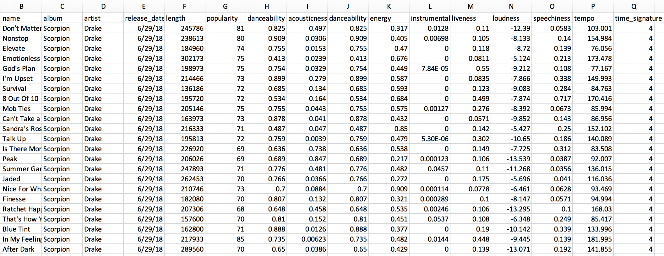
With the list of track ids, we can now loop over each id and obtain track information such as track name, album, release date, length, and popularity. More importantly, Spotify’s API allows us to extract a number of “audio features” such as danceability, energy, instrumentalness, and tempo. Without going into how these measures are determined, we’ll use them to understand how Drake’s style has evolved over time.

We’ll now loop over the tracks, applying the function, and save the dataset to a .csv file.

Here’s what the raw dataset looks like:

You can find the complete script to obtain this data here or download the dataset here.

Analyzing the Data

Let’s quickly clean a few variables in preparation for analysis. We’ll first convert the song length from milliseconds to minutes. Second, since the artist field captured the principal song artist, let’s create a boolean variable called “feature” which indicates whether or not Drake is the principal artist. Let’s also create a “year” variable using the release date for easy aggregation and grouping. Finally, we’ll reference the Drake discography Wikipedia page to create a “type” variable to distinguish between singles, extended plays (EP), mixtapes, studio albums, and feature tracks.

And now for some analysis. To begin, I’ve embedded a Tableau worksheet below which provides an overview of each Drake song for four core measurements:  danceability, energy, speechiness, and tempo.

This worksheet allows you to filter by type and to highlight a track within that type. I’d recommend clicking on the “expand” symbol in the lower right-hand corner for a better look.

A quick description of these four audio features, from the Spotify API Endpoint Reference:

Danceability: Describes how suitable a track is for dancing based on a combination of musical elements including tempo, rhythm stability, beat strength, and overall regularity. A value of 0.0 is least danceable and 1.0 is most danceable.

Energy: A measure from 0.0 to 1.0 and represents a perceptual measure of intensity and activity. Typically, energetic tracks feel fast, loud, and noisy. For example, death metal has high energy, while a Bach prelude scores low on the scale.

Speechiness: Detects the presence of spoken words in a track. The more exclusively speech-like the recording (talk show, audiobook, poetry), the closer to 1.0 the attribute value. Values between 0.33 and 0.66 describe tracks that may contain both music and speech, either in sections or layered, including such cases as rap music.

Tempo: The overall estimated tempo of a track in beats per minute (BPM).

Tracks Over Time

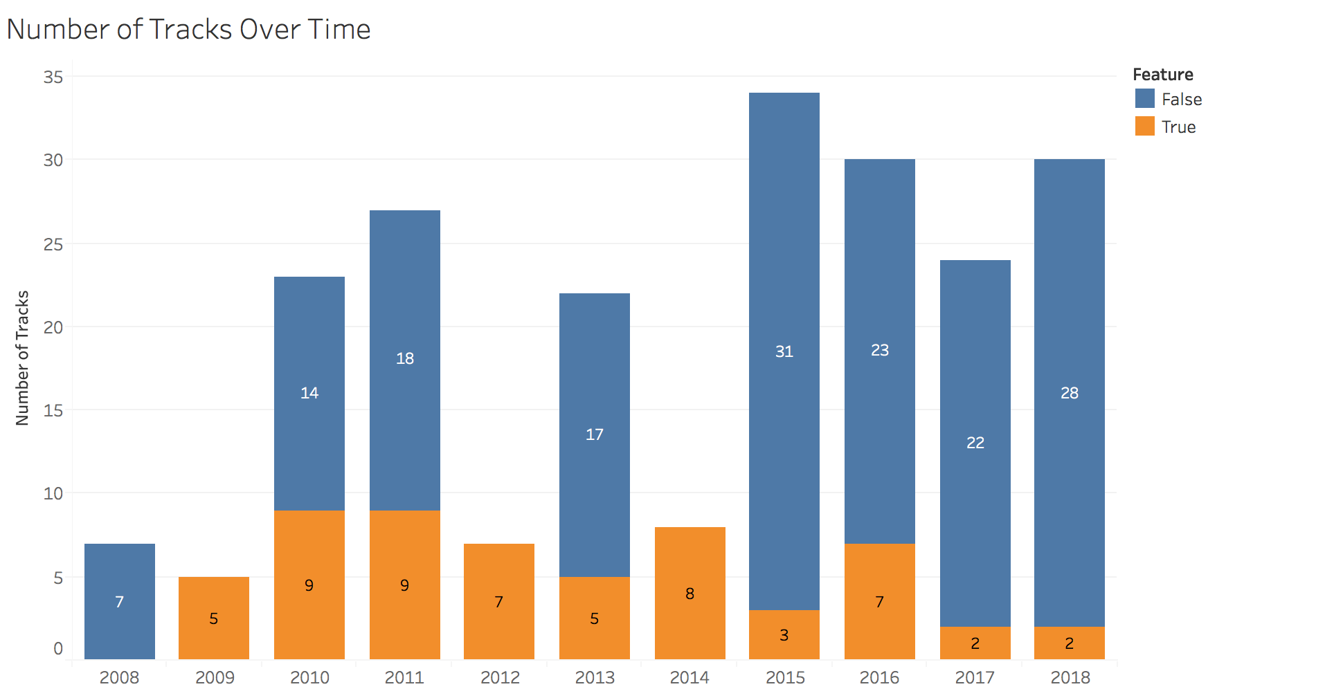
With those definitions clarified, let’s move onto a few visualizations. We’ll start with the number of tracks over time.

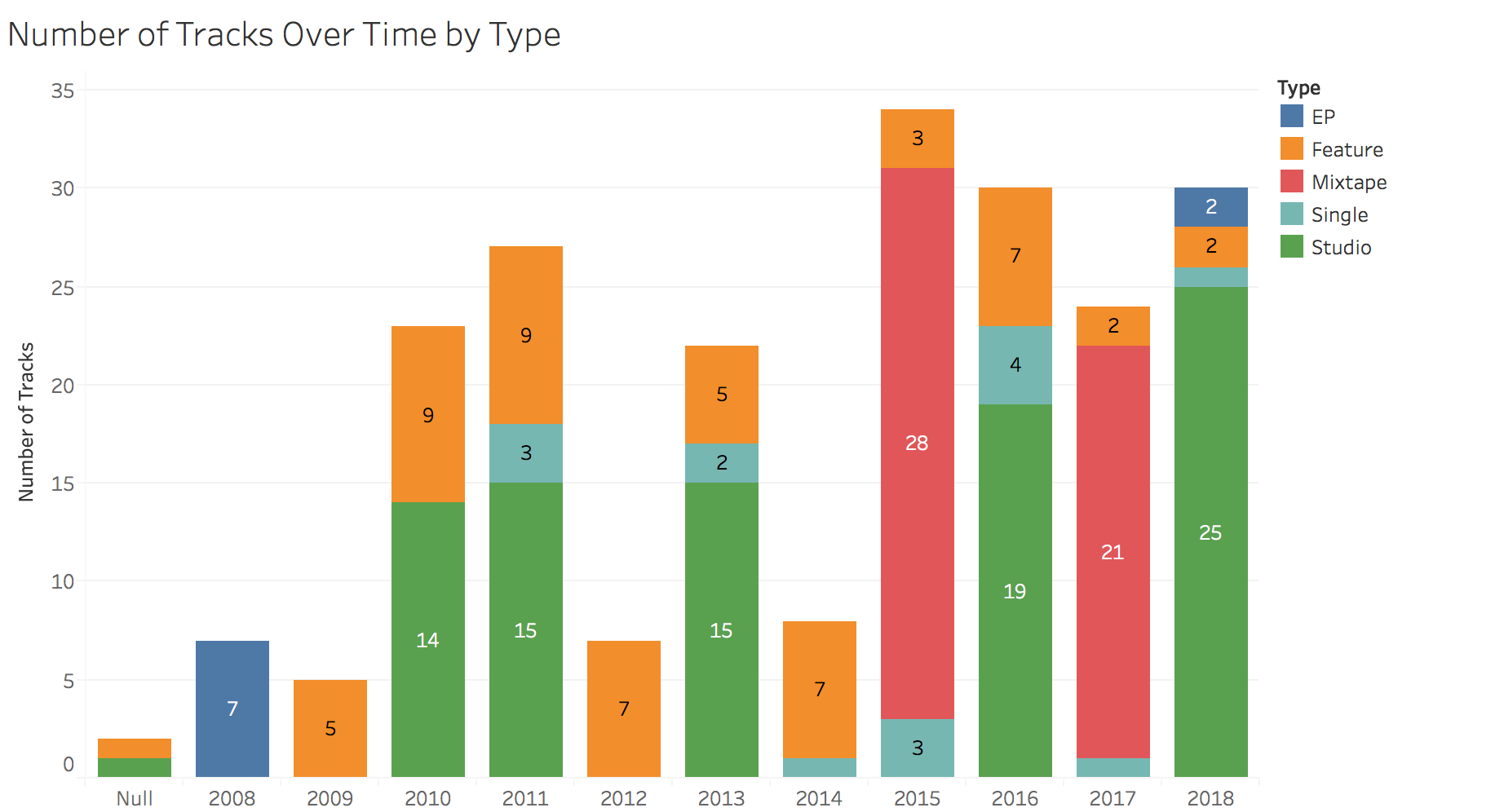
In this chart, we see that Drake has provided fans a fairly constant stream of new jams since 2008. In 2012 and 2014, Drake only jumped onto other artists’ song, releasing none of his own. In 2015, Drake blessed us with a doubleheader: If You’re Reading This It’s Too Late and What a Time to Be Alive plus additional singles and features for a total of 34 songs.

This can be seen more clearly in the next chart:

tracks-over-time-type

Track Length

I recently read a Pitchfork article (highly recommended, great visualizations) that analyzed the length of hip-hop records over the last 30 years. Drake is notorious for long albums, with his latest double-sided project coming in just under 90 minutes. Keeping in mind that there may be a strategic, streaming-oriented purpose, let’s take a look at how both album length and song length have trended over time.

The answer to the question posed in that Pitchfork article, “Are Rap Albums Really Getting Longer?” is abundantly clear here, at least in Drake’s case. His five studio albums have each progressively become longer. Some might call this a blessing, others a curse. What about average track length?

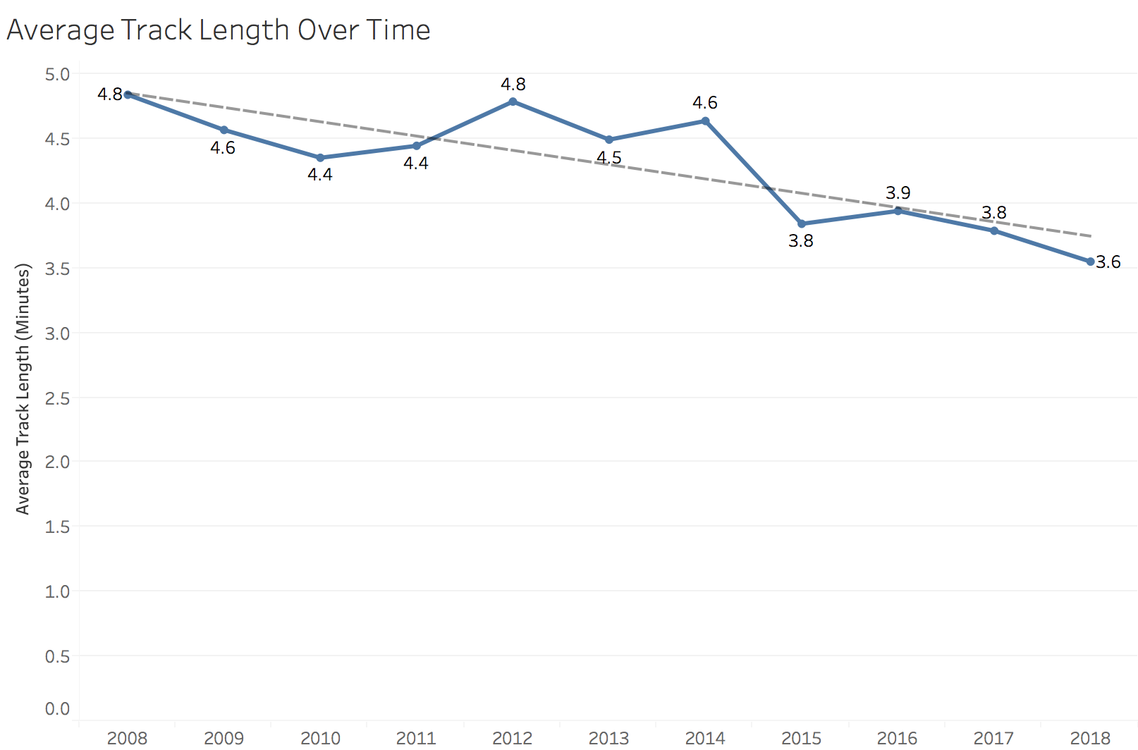
While Drake’s albums appear to be getting longer, his songs are, on average, getting shorter. Over the past decade, average song length has decreased more than a minute, from 4.8 minutes in 2008 to 3.6 minutes in 2018. Maybe this is another effect of the transition to streaming, as music streaming is now the industry’s biggest revenue source.

Danceability & Energy

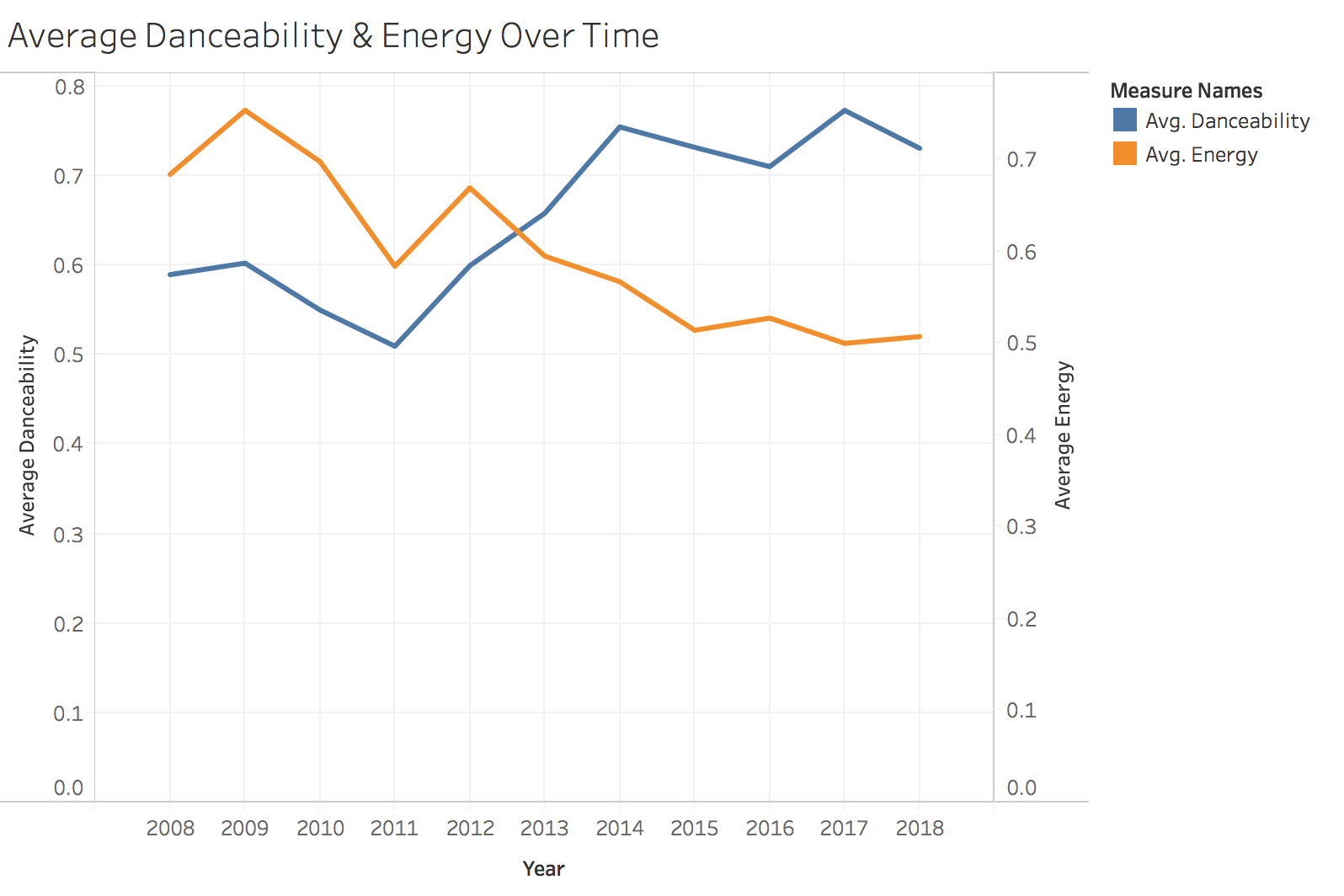
It’s pretty common for artists to “go pop” on the road to wider reach and popularity. Measuring the danceability metric for Drake’s songs over time might be a good way to test for a shift towards pop appeal. Shown below is average danceability and energy over time.

There’s a pretty clear upward trend in danceability, with a simultaneous decline in energy.

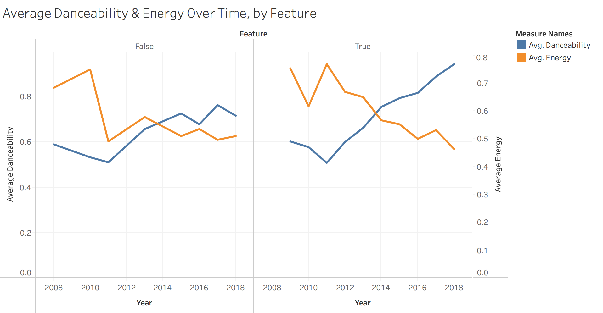
This holds true when we separate songs Drake is featured on versus his own, but his more pronounced on featured songs.

Top Collaborators

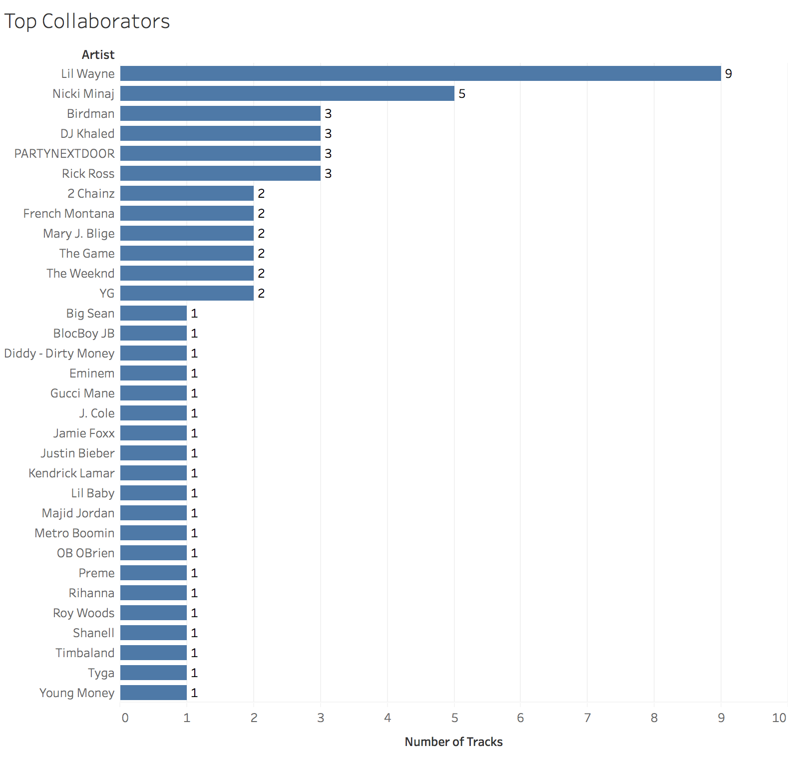
Finally, who does Drake like to work with? Here we measure the number of features by artist.

top-collaborators

The top three artists are all current or former Young Money acts. Beyond that, it’s clear Drake has worked with artists across a large spectrum of rap and R&B artists, from Rick Ross to Jaime Foxx.

Conclusion

APIs can be a great source of unique and interesting datasets. In addition to the information presented here, I’d be interested in expanding the dataset to include song recording location, principal producer, lyrical content, and the number of streams the track has obtained.

You can find the full, interactive version of the Tableau charts here and the dataset here.

css.php