python Archives - Page 2 of 2 - Unboxed Analytics

Analyzing Drake’s Catalog Using Spotify’s API

I’ve been a Drake fan since 2009 when I first heard “Best I Ever Had” from So Far Gone. Over the last decade, I’ve watched Drake transform into a global rap and pop superstar. This weekend I saw Drake live in Brooklyn as part of the Aubrey & the Three Migos tour. What better way to celebrate than by analyzing his catalog using Spotify’s API? I’ve broken the celebration into two parts, getting the data and analyzing the data. Click here if you’d rather skip the code and jump into the analysis.

Getting the Data

In this post, I use Spotipy, “a lightweight Python library for the Spotify Web API”. Let’s start by calling the necessary libraries.

Next, we need to authenticate and connect to the API. To do so, we need a “client id” and “client secret”. To obtain them, visit the Spotify Developer Dashboard here and create an application. In the code snippet below, replace the client id and client secret variables with your own.

There are a few potential ways to create a dataset of Drake’s catalog. We could have first obtained a list of the artist’s albums and then looped through each album track. Instead, I used a playlist by ‘100 percent’ which claims to have, “all of Drake, all in one place.” This collection of 219 songs (15+ hours) contains “every appearance currently on Spotify updated with each new release.” Great! We’ll now write a function to retrieve the ids for each track of this playlist.

With the list of track ids, we can now loop over each id and obtain track information such as track name, album, release date, length, and popularity. More importantly, Spotify’s API allows us to extract a number of “audio features” such as danceability, energy, instrumentalness, and tempo. Without going into how these measures are determined, we’ll use them to understand how Drake’s style has evolved over time.

We’ll now loop over the tracks, applying the function, and save the dataset to a .csv file.

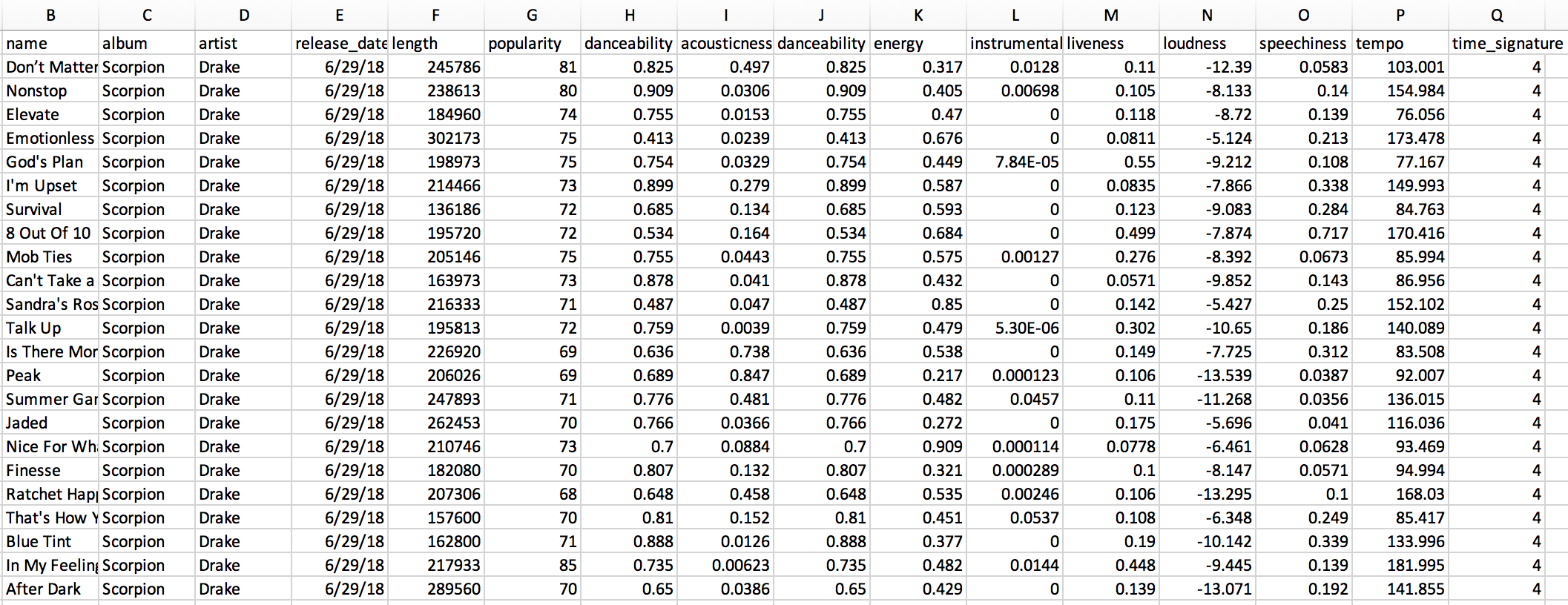
Here’s what the raw dataset looks like:

You can find the complete script to obtain this data here or download the dataset here.

Analyzing the Data

Let’s quickly clean a few variables in preparation for analysis. We’ll first convert the song length from milliseconds to minutes. Second, since the artist field captured the principal song artist, let’s create a boolean variable called “feature” which indicates whether or not Drake is the principal artist. Let’s also create a “year” variable using the release date for easy aggregation and grouping. Finally, we’ll reference the Drake discography Wikipedia page to create a “type” variable to distinguish between singles, extended plays (EP), mixtapes, studio albums, and feature tracks.

And now for some analysis. To begin, I’ve embedded a Tableau worksheet below which provides an overview of each Drake song for four core measurements: danceability, energy, speechiness, and tempo.

This worksheet allows you to filter by type and to highlight a track within that type. I’d recommend clicking on the “expand” symbol in the lower right-hand corner for a better look.

A quick description of these four audio features, from the Spotify API Endpoint Reference:

Danceability: Describes how suitable a track is for dancing based on a combination of musical elements including tempo, rhythm stability, beat strength, and overall regularity. A value of 0.0 is least danceable and 1.0 is most danceable.

Energy: A measure from 0.0 to 1.0 and represents a perceptual measure of intensity and activity. Typically, energetic tracks feel fast, loud, and noisy. For example, death metal has high energy, while a Bach prelude scores low on the scale.

Speechiness: Detects the presence of spoken words in a track. The more exclusively speech-like the recording (talk show, audiobook, poetry), the closer to 1.0 the attribute value. Values between 0.33 and 0.66 describe tracks that may contain both music and speech, either in sections or layered, including such cases as rap music.

Tempo: The overall estimated tempo of a track in beats per minute (BPM).

Tracks Over Time

With those definitions clarified, let’s move onto a few visualizations. We’ll start with the number of tracks over time.

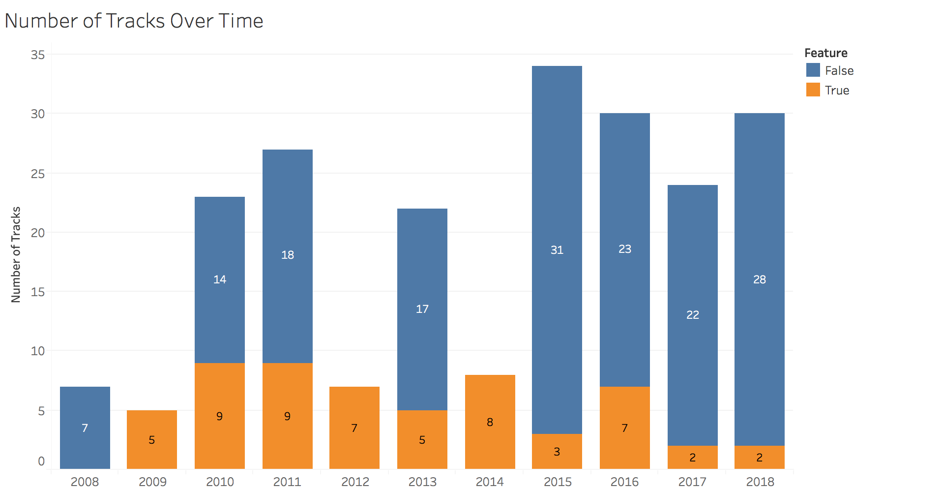
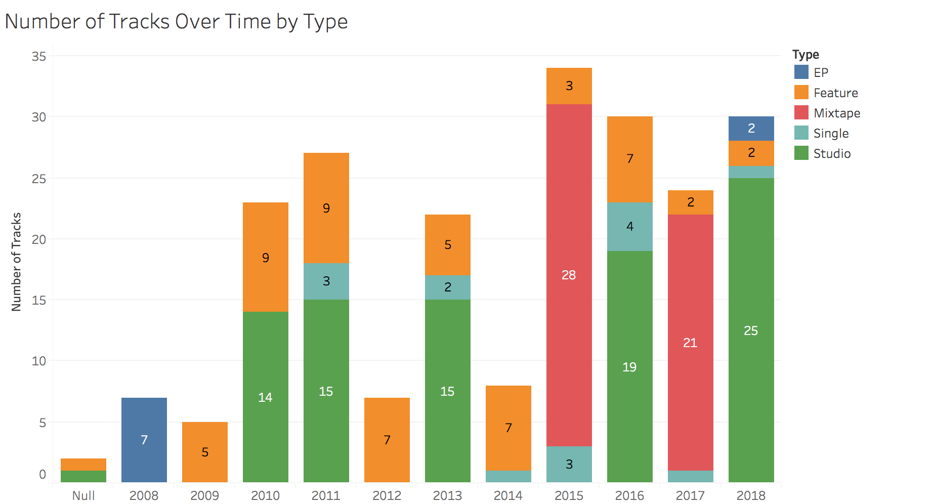
In this chart, we see that Drake has provided fans a fairly constant stream of new jams since 2008. In 2012 and 2014, Drake only jumped onto other artists’ song, releasing none of his own. In 2015, Drake blessed us with a doubleheader: If You’re Reading This It’s Too Late and What a Time to Be Alive plus additional singles and features for a total of 34 songs.

This can be seen more clearly in the next chart:

Track Length

I recently read a Pitchfork article (highly recommended, great visualizations) that analyzed the length of hip-hop records over the last 30 years. Drake is notorious for long albums, with his latest double-sided project coming in just under 90 minutes. Keeping in mind that there may be a strategic, streaming-oriented purpose, let’s take a look at how both album length and song length have trended over time.

The answer to the question posed in that Pitchfork article, “Are Rap Albums Really Getting Longer?” is abundantly clear here, at least in Drake’s case. His five studio albums have each progressively become longer. Some might call this a blessing, others a curse. What about average track length?

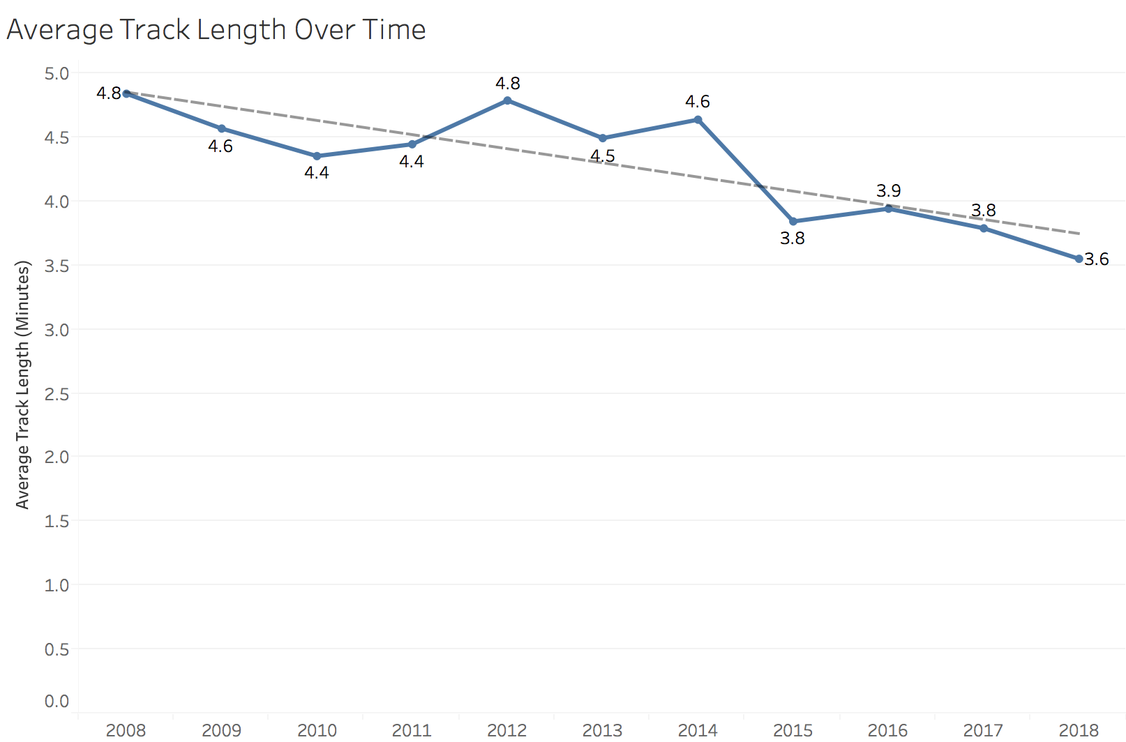
While Drake’s albums appear to be getting longer, his songs are, on average, getting shorter. Over the past decade, average song length has decreased more than a minute, from 4.8 minutes in 2008 to 3.6 minutes in 2018. Maybe this is another effect of the transition to streaming, as music streaming is now the industry’s biggest revenue source.

Danceability & Energy

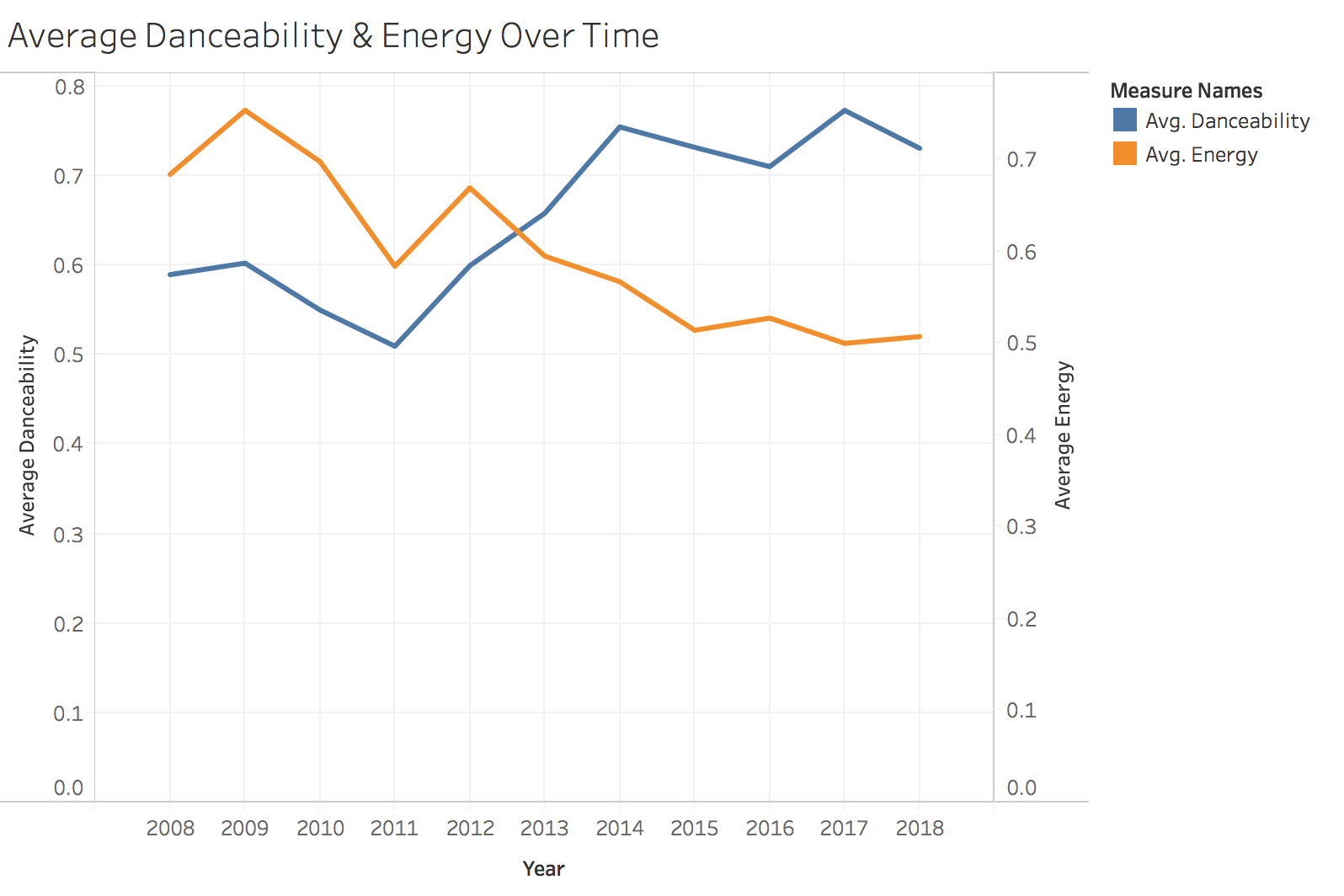
It’s pretty common for artists to “go pop” on the road to wider reach and popularity. Measuring the danceability metric for Drake’s songs over time might be a good way to test for a shift towards pop appeal. Shown below is average danceability and energy over time.

There’s a pretty clear upward trend in danceability, with a simultaneous decline in energy.

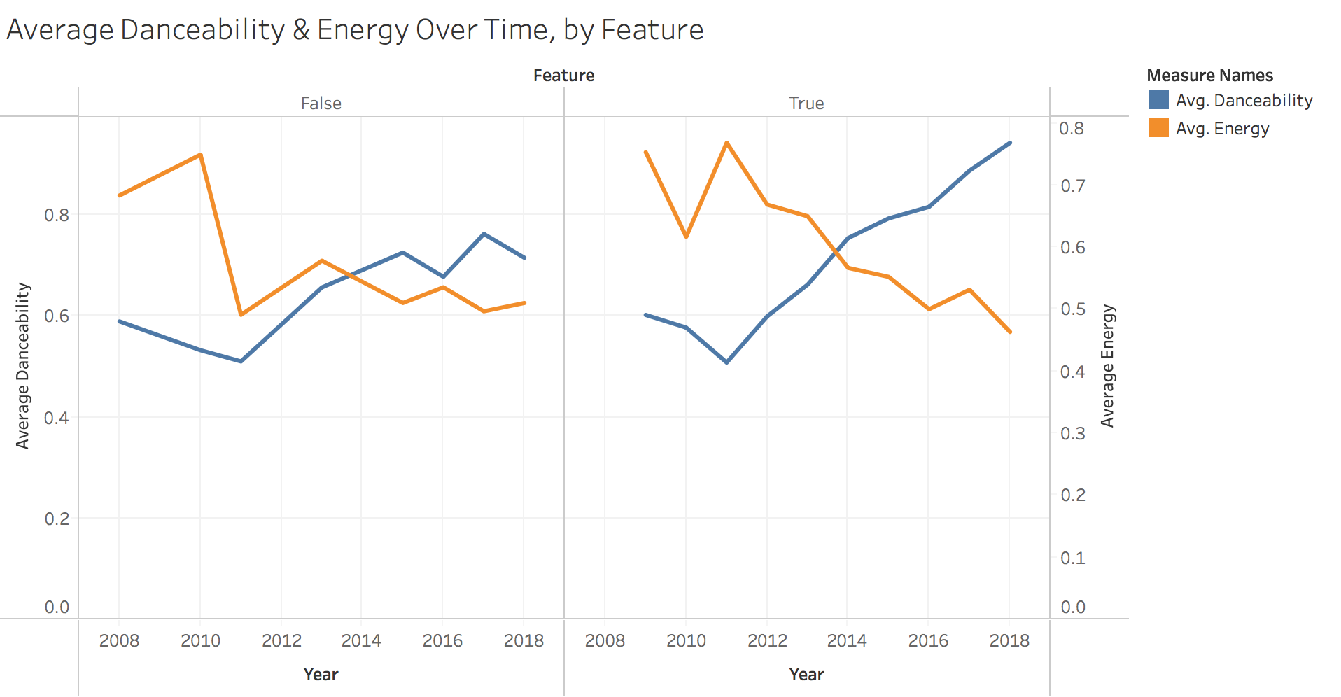
This holds true when we separate songs Drake is featured on versus his own, but his more pronounced on featured songs.

Top Collaborators

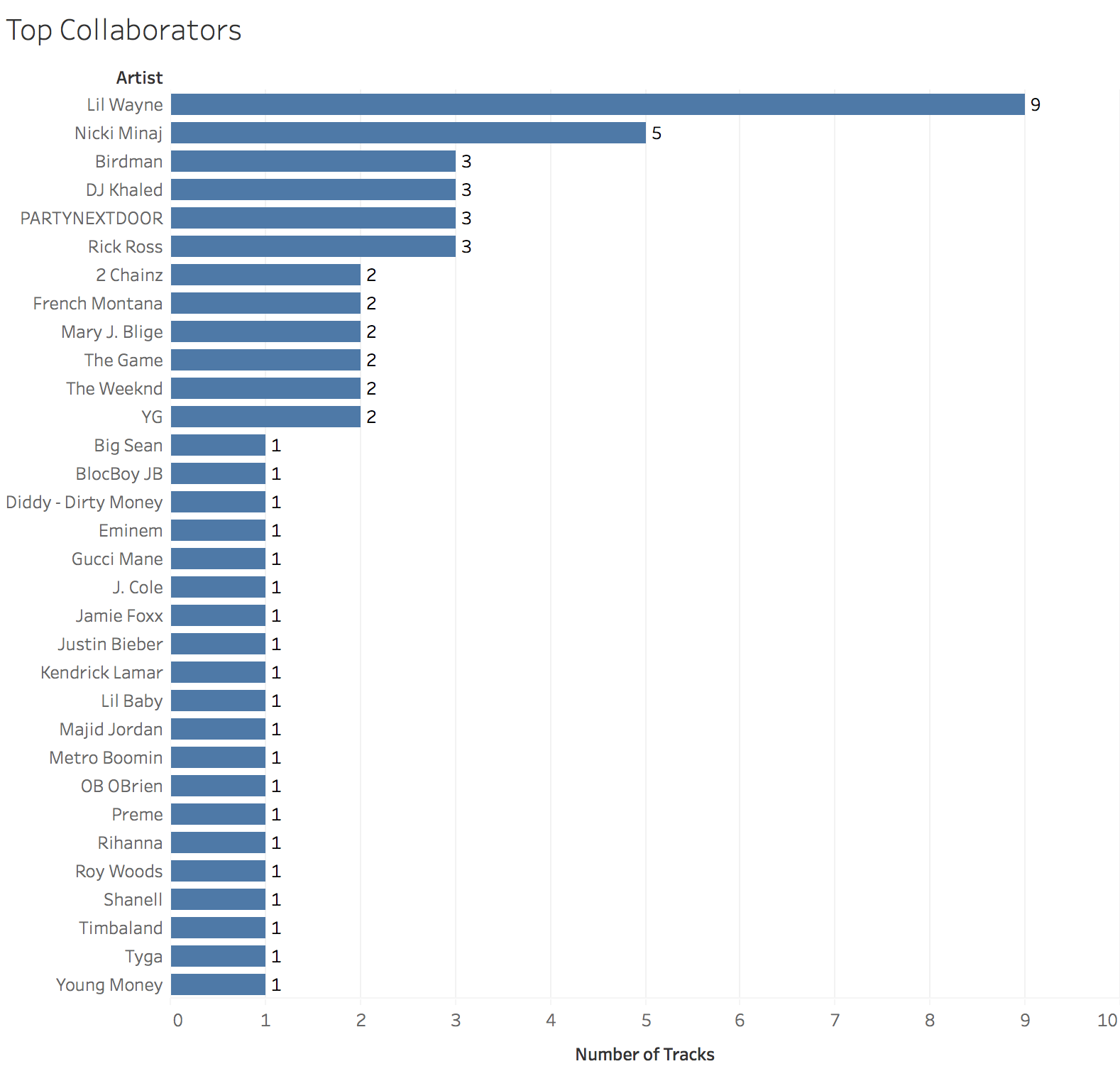
Finally, who does Drake like to work with? Here we measure the number of features by artist.

The top three artists are all current or former Young Money acts. Beyond that, it’s clear Drake has worked with artists across a large spectrum of rap and R&B artists, from Rick Ross to Jaime Foxx.

Conclusion

APIs can be a great source of unique and interesting datasets. In addition to the information presented here, I’d be interested in expanding the dataset to include song recording location, principal producer, lyrical content, and the number of streams the track has obtained.

You can find the full, interactive version of the Tableau charts here and the dataset here.

The Hunt for Housing in NYC: A Data-Driven Approach

This summer my wife and I relocated to New York City in preparation for the start of my new job. Housing in Manhattan and the surrounding boroughs is notoriously expensive, so I decided to pursue a data-driven approach to our apartment search. I wrote a Python script to scrape 9,000+ apartment listings on Craigslist for zip codes in the five boroughs: Manhattan, Bronx, Brooklyn, Queens, and Staten Island. I then visualized the median rent by zip code in Tablaeu. Check out the dashboard here!

Gathering the Data

Before digging into some housing insights, let’s walk through the process used to obtain the data. First, I obtained data about the organization of New York City’s boroughs, neighborhoods, and zip codes from a New York State Department of Health website. I then leveraged the structure of Craigslists’s URLs to construct a vector of links to search for apartments in each of the zip codes. Here’s what the URL to search for apartments with the zip code 10453 looks like:

https://newyork.craigslist.org/search/aap?postal=10453

Let’s see what that looks like in code.

The ‘nyc-zip-codes.csv’ file referenced above can be found here. Next, I wrote a function to extract the pertinent information from each listing from each of these links. I extracted the listing title, posting date, monthly rent, and the number of bedrooms, when available.

This is what the function returns when fed the sample link for zip code 10453.

At this point, we just need a way to loop through each zip code and compile the data the function returns.

After cleaning the data and removing duplicates, we have about 9,400 listings to work with.

Analyzing the Data

Let’s start with the big picture and then zoom in. Below we have the median rental price of listings by borough. Manhattan is by far the most expensive place to live, followed in distant second by Brooklyn. Queens, Staten Island, and the Bronx are actually somewhat comparable, with median rent in Queens only $250 higher than median rent in the Bronx.

How does rent vary in the five boroughs by the number of bedrooms the unit has? Filtering the data to include only units with 1 to 4 bedrooms, Manhattan is still the most expensive for each number of bedrooms.

Note that the bracketed, italicized numbers above show the number of listings for each borough and bedroom combination.

My wife and I had hoped to find a 2-bedroom apartment in a safe neighborhood with a 30-minute commute to Midtown for $2,000 or less. But, as you can see in the image below depicting median 2-bedroom rent by zip code in Queens, that may be a tough find!

Now, what else would I have liked to add to this analysis? Since one major consideration in the hunt for housing is commute time, how about a distance-adjusted median rental price metric for each zip code? This is something I’ll tackle in a future post.

Conclusion

Ultimately, my wife and I found housing in Scarsdale through a family friend and didn’t end up living in any of the five boroughs! Luckily, by feeding the script a different set of zip codes and modifying the Craigslist URL structure, I’ll be able to replicate this data-driven process in future apartment searches.

Find the complete code here, hosted as a Gist on GitHub.

Check out my other data projects here.

Complete Python Selenium Web Scraping Example

Introduction

I recently listed a couple of items for sale on a Craigslist-like site called KSL Classifieds. It’s a rich marketplace to buy and sell almost anything. This is what a listing looks like:

I instinctively started thinking about how to collect information about listings in this marketplace in a systematic way. Why might this kind of autotomized data collection be valuable? Here are two possible use cases:

Listing optimization. We could analyze how features of a listing (number of pictures, description length, listing category/subcategory, etc.) are related to outcomes such as the number of views, if the item is “favorited” by users, or whether or not the item was sold. This kind of data-driven listing optimization could drive sales for sellers.
Automated Item Search. There’s value for buyers as well. Suppose I’m looking for something specific, like a wakeboard for family boating outings. I could easily automate a script to scrape all wakeboard listings daily and send me the information via email, simplifying the search process.

Walkthrough

Let’s jump into the walkthrough. At a high level, we know we want our web scraping script to take a KSL Classified URL as input and output a CSV containing neatly-arranged data from each listing. Here’s what the starting page might look like:

Given this page, we need to find all the links to listings, navigate to each listing page, and then extract the desired information. Each listing contains the following features:

Title
Location (City, State)
Time Posted
Price
Number of Views
Number of Favorites
Description
Seller Information

With that as background, let’s get into the code. We’ll start by calling the libraries.

Next, we’ll write a function to extract all the listing links from a search result page like the one above.

Note that I’m using “ChromeDriver”. It can be downloaded here. Below is what the output of our function looks like. We now have a vector of links to specific listings.

Now we need to iterate through each of these listings and extract the desired information. Below is a function called getListingContent() which takes a listing link and return the title, location, time since listing posting, price, views, favorites, description, seller, and the listing URL.

Again, here’s what the output of this function would look like:

Pretty slick eh? Now let’s combine these two functions!

Here we’re only going to loop through the first ten of the listing links gathered by getListingLinks(). After the loop, we’ll neatly arrange the extracted data into a Pandas DataFrame.

To finish things off, we’ll clean the data. This includes reformatting the “price” variable and changing “views” and “favorites” from strings to numbers.

Finally, let’s tie it all together with the main() function:

Nice work! We can now pass a link to main() and it will generate a tidy CSV file with information about the listing from that page. You can find the complete scraper code here. Below are some resources that proved helpful to me in creating this example: