
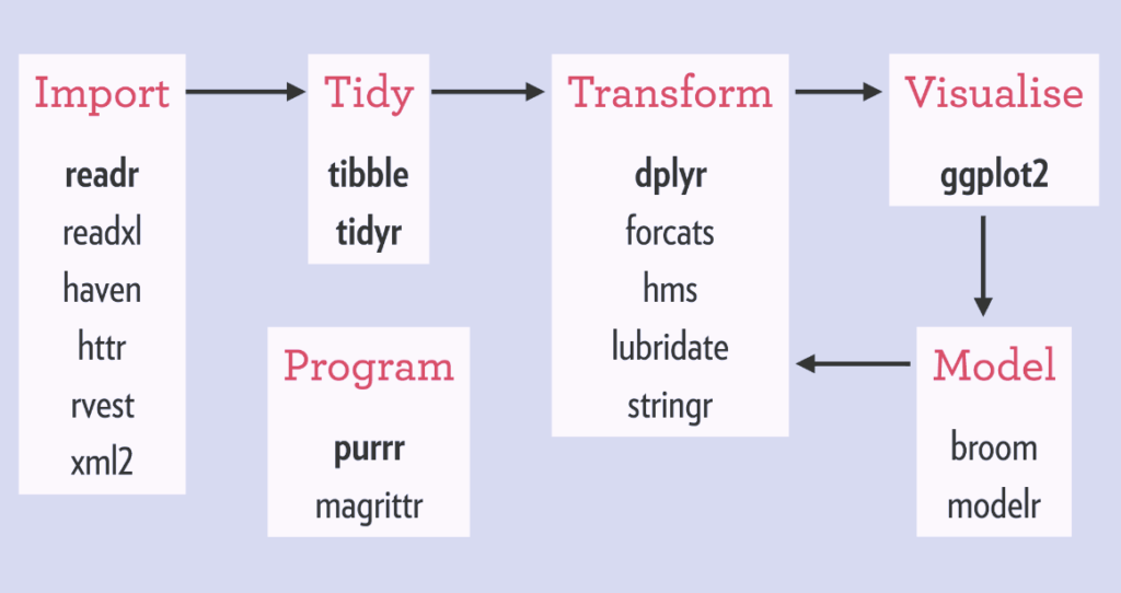
Inspired in part by Python’s Beautiful Soup, the R package rvest makes it delightfully easy to scrape data from the web. As part of the Tidyverse collection of packages, rvest fits nicely within the broader data workflow:
In this post I’ll walk through an example of using rvest to compile a dataset of NBA player salaries. To follow along, create a free RStudio Cloud account to write and run R code and bookmark the SelectorGadget tool to help identify HTML/CSS tags.
Background
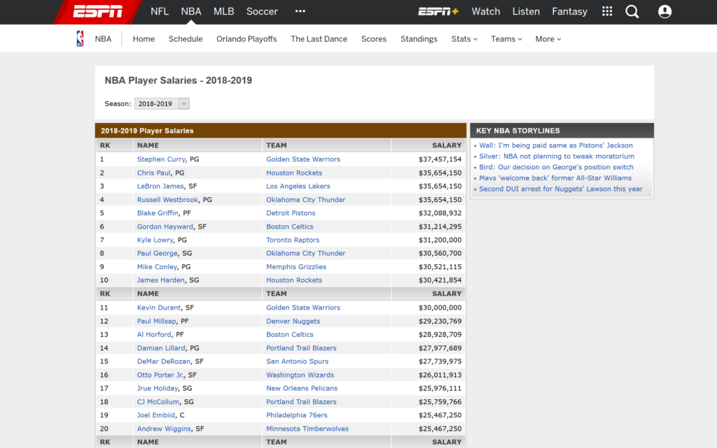
Professional athletes are paid handsomely for their highly-specialized skill sets, and NBA players are no exception. Take Steph Curry, the highest-paid player during the 2018-2019 season. During that season he brought in a cool $37M in salary.

highest player wages worldwide (source, image source)
ESPN publishes annual salary data going back to the 1999-2000 season. Rather than manually copying this data, which is spread across hundreds of web pages, we can write a script to compile the data automatically using rvest. The data can then be used to explore variation in salary over time, by team, and by position.
Page Structure
The first step in any web scraping project is to become familiar with the target site URL structure. In this case, ESPN has a different page for each season. For example, the link below contains the player salaries for the 2018-2019 season:
http://www.espn.com/nba/salaries/_/year/2019
Within each season, the salaries are spread across several sub-pages, with 40 players listed on each sub-page:
http://www.espn.com/nba/salaries/_/year/2019/page/2
This means our code will need to dynamically determine the number of sub-pages to loop through when scraping the player salaries from each season.
Code Walkthrough
With that background, let’s dive into the code! To get started, we’ll need three packages: rvest, tidyverse, and stringr:
Next, we’ll define a vector of season URLs to loop over:
Next comes the bulk of the code required to perform the scraping. Here we loop over each of the season URLs. By extracting the text from the .page-numbers element on each page, we can dynamically determine the number of sub-pages for each season.
The html_table() command from the rvest package detects and extracts the table of salaries from each sub-page.
The last step is to clean the raw scraping output by adding column names, removing extra rows, and splitting the “name” and “position” fields into two columns, since they were stored as a single column in the ESPN tables, separated by a comma.
The final dataset has 9,456 rows. Below are the first 10:
| rank | name | position | team | salary | season |
|---|---|---|---|---|---|
| 1 | Shaquille O'Neal | C | Los Angeles Lakers | 17142000 | 2000 |
| 2 | Kevin Garnett | PF | Minnesota Timberwolves | 16806000 | 2000 |
| 3 | Alonzo Mourning | C | Miami Heat | 15004000 | 2000 |
| 4 | Juwan Howard | PF | Washington Wizards | 15000000 | 2000 |
| 5 | Scottie Pippen | SF | Portland Trail Blazers | 14795000 | 2000 |
| 6 | Karl Malone | PF | Utah Jazz | 14000000 | 2000 |
| 7 | Larry Johnson | F | New York Knicks | 11910000 | 2000 |
| 8 | Gary Payton | PG | Seattle SuperSonics | 11020000 | 2000 |
| 9 | Rasheed Wallace | PF | Portland Trail Blazers | 10800000 | 2000 |
| 10 | Shawn Kemp | C | Cleveland Cavaliers | 10780000 | 2000 |
Visualization
With the hard part out of the way, let’s quickly explore the trend in player salaries. We’ll visualize the distribution of salary by season:
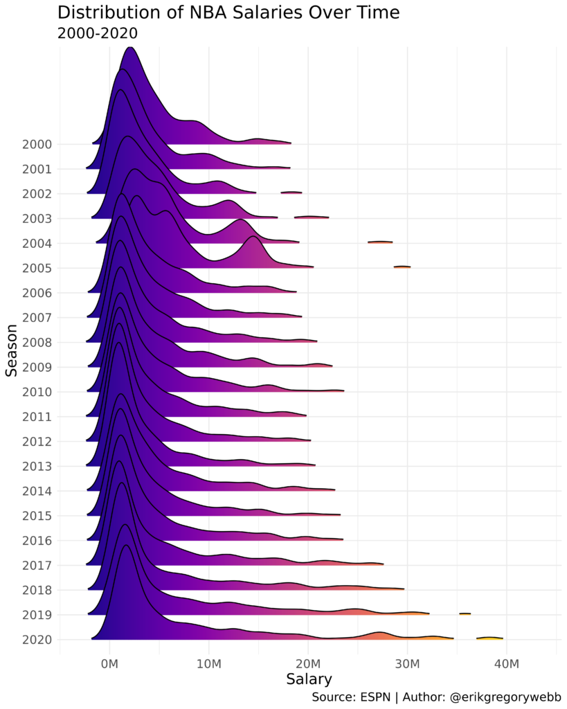
Notice how the right tail has grown over time. It appears that most of the growth in average player salary is being drive by salaries paid to superstars. This observation is consistent with a similar analysis of NBA salaries done by Dimitrije Curcic.
“The average salary in the NBA has increased more than 7x since the 1990-91 season. Median salary has slower growth than the average; this could suggest that the financial gap between the top talents and the rest is getting larger.”
Here’s the code used to create the chart.
Web scraping is an important tool for data analysis because it enables data collection at scale. Rvest streamlines the process, allowing you to quickly create novel datasets for analysis, like NBA player salaries.